User Guide

This page provides a step-by-step guide for using the TJPDC’s REF dataset to evaluate projects. The tool can be used for two main functions:

1. The first is to evaluate a projects potential impact by providing a project sore (or average Eco-Logical score). This score can be then compared across a set of alternatives to help identify the project with the least potential for habitat and environmental impacts. The Project Scoring Guide walks through this process.
2. The second function of the tool is its ability to identify a least damaging route across the REF automatically. This process is useful for identifying the least damaging route, which can be used as a benchmark for other alternatives. The Least Cost Path Guide walks through this process.

To perform the steps described in the guide you must have a copy of ESRI ArcGIS 10.1 Desktop (or higher) and the ArcGIS for Desktop Spatial Analyst extension. You will also need a copy of the TJPDC regional Ecological framework basemap.

• Open ArcMap and check that you have the Spatial Analyst Extension turned on. To do this go to the Customize menu and click on extensions. Next make sure that there is a check box next to Spatial Analyst in the list.
• Use the add data button to open the REF dataset.
• Apply the appropriate color ramp. After opening, right click on the REF dataset (located in the Table of Contents on the left side of the GIS window). Click properties, then click on the Symbology tab. Click the color ramp dropdown and select an appropriate single color ramp. In this example we are using a shade of green. Hit the OK button to exit the Layer Properties dialog box.
• Apply the proper coordinate system. Right click anywhere in the data frame and select data frame properties. Navigate to the Coordinate System Tab and set the coordinate system to: NAD_1983_StatePlane_Virginia_South_FIPS_4502_Feet. Hit OK to exit the Data Frame Properties dialog box.

You are now ready to add the project to be analyzed. In this case, we will be analyzing a fictitious rail link between Scottsville and the Charlottesville. Click the add data button to open your project area. In this example we are using a 200 foot wide rail right of way. Note: for best results your project footprint should be in raster and not vector format.

• Once you have your project added you are ready for the analyses. To begin, click on the Geoprocessing menu and select Arc Toolbox. This will bring up the Arc Toolbox tree.
  • In the tree navigate to the Spatial Analyst Tool and click on the + button to open the toolbox.
  • Click the + next to the Zonal toolbox and then click on the Zonal Statistics as Table tool. This will bring up the Zonal Statistics as table Dialog Box.
• In the tool dialog, you will first select your Input Raster.
  • From the dropdown list, select the file that represents your project. In this case, it is the Scottsville_Cvill_Rail_200.tif file. You can leave the Zone filed on the default value.
  • Select the REF dataset file from the dropdown list for the Input Value Raster field. In this example, we are using Final_State_Plane.tif.
  • In the output table, select an appropriate directory to name and save the output table that will be generated. Note: this file will be added automatically to your Table of Contents when the tool finishes processing.
• Set the processing extent. Before running the analyses, click on the Environments button. This will bring up the Environments Settings window.
  • Click on Processing Extent and set the extent to be the same as the REF Raster. In this example we use Same As Layer Final _State_Plane.tif.
  • Click on Raster Analysis and set the Cell Size to be the same as the REF. Again, in this example we select Final _State_Plane.tif. Click OK to close the window.
• You can now hit OK to run the Tool.
• View the Results. When the tool finishes a new table will be added to your table of contents.
  • Open the table to view the results. The key figures are the Mean, and the sum, The mean can be used for a quick comparison to the distribution of values across the REF. The key figure is the “SUM” which once normalized by project area can provide a comparable REF Conflict Score. For example the fictitious rail project used in the analyses has an area of 487.3 acres and has a “SUM” of 1620. 1620/487.3= a REF Conflict score of 3.3.

We will continue to use the fictitious rail link project for this example. To begin the analyses repeat the steps detailed in preparing for GIS analyses. Once you have completed these steps you are ready to add your project start and end point data. In this example, we are using points that represent two new train stations (Charlottesville and Scottsville).

• To begin the analyses click on the Geoprocessing menu and select Arc Toolbox. This will bring up the Arc Toolbox tree. In the tree navigate to the Spatial Analyst Tool and click on the + button to open the toolbox.
  • Click the + next to the Distance Toolbox and select the Cost Distance tool. This will open up the cost distance tool dialog box. In the Input, raster or feature source data field select your “end” point. Note: it doesn’t matter which one you use for your start and end points, you just need to keep track so you can use the other point in part 2 of the analyses. In this example, we select Charlottesville.
  • Select the REF as your Input cost raster. When this tool runs, it will create two new datasets, which are required in step two. In the Output distance raster field, navigate to a folder to save the output. Give it a name like distance_Rast.tif. Note: Remember to include the .TIF extension if you want your rasters saved in that format. Now do the same for the Output backlink raster.
• Before running the analyses, click on the Environments button. This will bring up the Environments Settings window.
  • Click on Processing Extent and set the extent to be the same as the REF Raster. In this example, we use same as Layer Final _State_Plane.tif.
  • Click on Raster Analysis and set the Cell Size to be the same as the REF. Again, in this example we select Final _State_Plane.tif. Click OK to close the window.
  • You can now hit OK to run the Tool. Note: processing can take an extended period of time. When the tool finishes you will have two new rasters in your table of contents. These rasters will be used in step two.

The least cost path analyses uses the two rasters generated in step one to calculate the least impactful project path based on distance and the values in the REF.

• To perform this step of the analyses, open Arc Toolbox by navigating to Geoprocessing menu and clicking on Arc Toolbox.
  • In the Arc Toolbox tree navigate to the Spatial Analyst Tool and click on the + button to open the toolbox.
  • Click the + Distance Toolbox and then click on Cost path, this will bring up the Cost Distance tool dialog box.
  • In the Input, raster or feature source data field select your “start” point.
  • From the dropdown select the other point from the one you used in step one. In the case of the example, we are using Scottsville.
  • Select the cost raster you created in step 1 from the Cost raster field dropdown. Leave the maximum distance blank and select your backlink raster from step 1. Set an output file location and name. Remember to use the TIF file extension.
• Before running the analyses, click on the Environments button. This will bring up the Environments Settings window.
  • Click on Processing Extent and set the extent to be the same as the REF Raster. In this example we use Same As Layer Final _State_Plane.tif.
  • Click on Raster Analysis and set the Cell Size to be the same as the REF. Again, in this example we select Final _State_Plane.tif. Click OK to close the window.
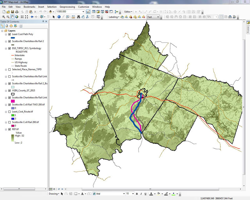
  • You can now hit OK to run the Tool. When finished the tool will add a new raster to your Table of Contents.

The new raster will contain three values 0, 1, 3. The least cost path line is represented by “3” value. To see it you will need to right click on the new raster and open the properties dialog box. Once open navigate to the Symbology tab and remove the 0 and 1 value from the list. Close the window to see your new least cost path. This line represents the potentially least ecologically impactful route.